Bitcoin Power Law Analysis Tutorial
1 Interactive Axis explorer
Generated by: btc_price_interactive_pl.py
Modification needed: Add actual price data to the interactive chart, possibly replace slider with range selector.
How robust is this power law relationship over different time periods? Use this interactive chart to change the range of dates used to fit the power law line. Observe how including or excluding certain periods of Bitcoin's history impacts the calculated trend.
5. Interactive Power Law Exploration
run btc_price_interactive_pl.py then come back
6. R-squared Heatmap
Generated by: btc_price_pl_compare_periods.py
This heatmap visualizes the R-squared values of the power law fit for all possible start years and period lengths. Brighter colors indicate higher R-squared values, representing a better fit. Remember to consider the effects of autocorrelation when interpreting these values, as data points closer in time are naturally more correlated.
8. Bitcoin Power Law Floor and Ceiling.
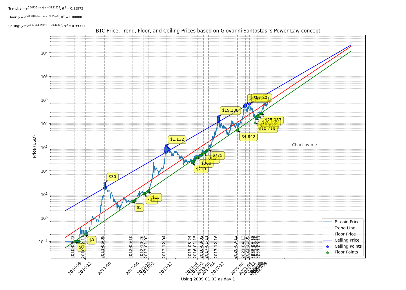
Generated by: btc_price_graph.py
The floor price is based on the assumption that in the long term, Bitcoin’s price follows a power law trend and cannot fall below a certain level.
The ceiling price is a less reliable trend line as the market tends to "overshoot" on the way up.
Future zoom
Zoomable Bitcoin Price History with Power Law Trends
Use the zoom controls to explore different time periods. The trend lines extend into the future for price projection analysis.
8. Time-Price Ratio Analysis
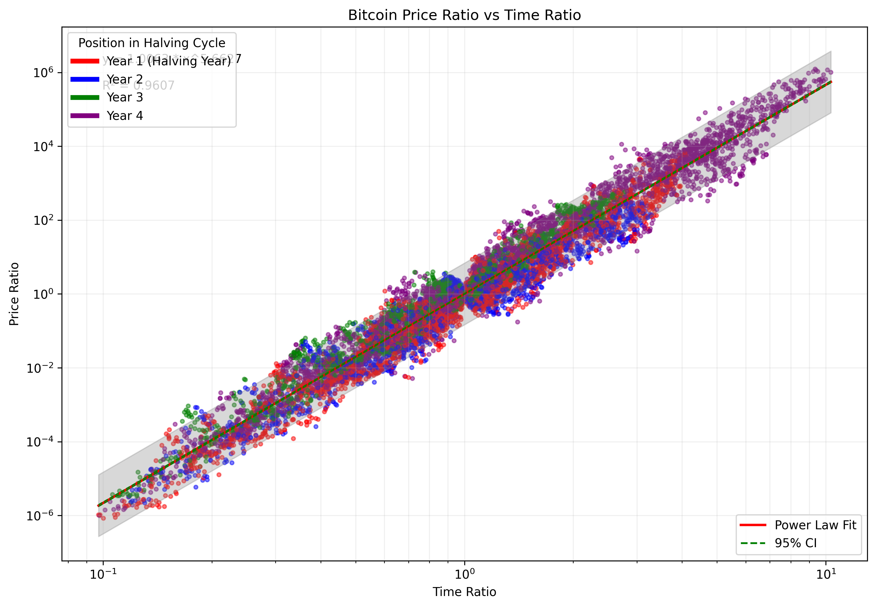
Generated by: btc_time_price_ratio_analysis.py
This scatter plot analyzes the relationship between time ratios and price ratios. Each point represents a pair of randomly selected dates (t1, t2), and shows how much time has elapsed (t2/t1) versus how much the price has changed (p2/p1). The power law fit line (and its confidence interval) helps quantify this relationship, providing further evidence of Bitcoin's power law price behavior. The colors represent the four years of the Bitcoin halving cycle.
9. Price History Relative to Floor
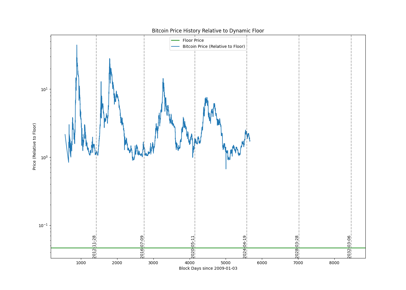
Generated by: btc_price_graph_flattened.py (Corrected filename and slight modification needed)
Filename should be: btc_price_history_relative_plot.png. The output needs slight modification to be saved as a PNG.
This chart shows the Bitcoin price relative to a dynamically calculated floor price. This floor price, derived from a robust power-law fit to the lowest historical prices, provides a baseline against which to measure price increases. The peaks (marked in red with confidence intervals) represent cycle highs relative to this floor, allowing for analysis of peak magnitude and timing. Linear and quadratic projections for peak height are shown as well.
10. Folded Price Cycles (4-Year Cycle Visualization)
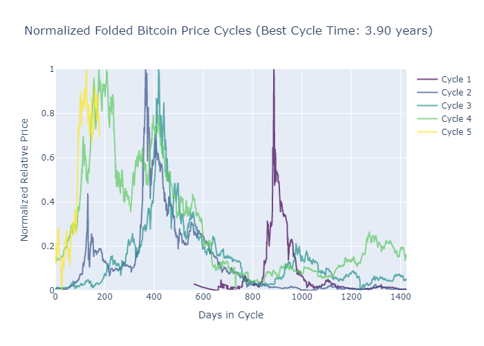
Generated by: btc_price_graph_flattened.py
This chart visualizes the price history of Bitcoin, with the price axis folded to show the 4-year cycle. The peaks (marked in red with confidence intervals) represent cycle highs relative to the floor price. The peaks are marked .
To visualize recurring cyclical patterns, the price history is "folded" over a 4-year period (approximating the Bitcoin halving cycle). This helps to identify similarities and deviations in price behavior across different cycles. The overlapping curves created by folding highlight consistent trends and patterns. Each curve represents a halving cycle or period of approximately four years, and these cycles are overlayed on each other. This visual clarifies the concept of cyclicality in the Bitcoin price history. Each cycle begins at the point of its respective halving. The folded cycles graph does an excellent job of clarifying whether the current price is high or low *relative to a similar point in previous cycles*.